
Mastering SQL Optimization: From Functional to Efficient Queries
Six Simple Yet Effective SQL Tips That Helped Me Reduce 50 Hours of Snowflake Query Time Every Day
SQL is probably the most fundamental technical skill every data analyst and data scientist should master. It’s usually part of the interview process, and we spend significant time coding in SQL at work to collect data. Without it, there is no analysis or machine learning models. However, writing a functional query is different from writing a good query.
At my recent job, we have over 1,000 queries scheduled on Airflow daily by our data scientists. I observed our Snowflake credits increased by 50% in just one year. When I volunteered to examine the top 10 credit usage queries, I soon realized there were numerous optimization opportunities, some quite simple. This article highlights six simple yet effective tips that helped me reduce SQL query running time by 50 hours daily. Some of them are extremely simple to apply, but remember, 20% effort in SQL optimization leads to 80% of performance improvements.
Note:
- This article is written for those who are already familiar with basic SQL grammar. If you are a fellow data analyst or data scientist who writes SQL daily but wants to improve your queries (and make your data engineer friends happy), this is for you!
- This article is based primarily on my experience with Snowflake SQL. While I focus on universally relevant tips, please remember that each data warehouse operates differently, so some tips may be less applicable to other platforms. Please try and compare query performance in practice.
Understand Your Query in Snowflake
Before diving into optimization techniques, it’s essential to understand the underlying mechanism of your query and identify the most resource-intensive parts.
Luckily, if you use Snowflake SQL at work, they have the invaluable Query Profile tool. Here are the steps:
- Go to the ‘History’ tab or the ‘worksheet’ page;
- Find the query you want to analyze and click on the Query ID;
- Go to the ‘Profile’ tab and read through the Operator Tree. This will show you all the specific operations the query took in sequence in the background, how long each took, the execution time breakdown, and the cost.
For example, in the below screenshot, you can see the Join step taking the longest time, followed by the Aggregate (SUM) operation.
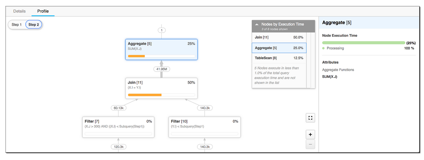
This tool is incredibly helpful for identifying inefficient query steps. When you try out the optimization tips below, you can also compare the query profile before and after to understand the underlying changes better.
SQL Query Dos and Don’ts
To explain the tips more easily, let’s assume we work at an e-commerce company with the following tables:
- users: a wide user-level table. Each row is a registered user on the e-commerce site. Columns include user_id (primary key), signup_time, and all sorts of demographic info (say, 20+ columns) like age, gender, country, billing_address, etc.
- products: a product-level table. Each row is a product we sell on the site. Columns include product_id (primary key), product_name, product_category, etc.
- orders: an order-level table. Each row is an order a user placed on the site. Columns include order_id (primary key), user_id (foreign key), order_time, etc. Let’s also assume it has a large column payment_information, storing a large JSON blob with credit card transaction data.
- ordered_products: a table at order x product level. It tells which products are included in each order. Columns include order_product_id (primary key), order_id (foreign key), product_id (foreign key), and price.
Now let’s talk about my top six simple yet effective SQL query optimization tips.
1. Only select the necessary columns
It is the easiest yet often overlooked tip, especially for data warehouses that use columnar storage like Snowflake. You should only select the columns you need, especially when dealing with large tables, running window functions, or multiple joins. Writing SELECT *is easy but can be very expensive and slow down your query. Optimizing column selection helps reduce computational resource usage and costs, and improves readability.
I was able to speed up a query 4x by simply specifying the columns I needed and leaving out the large JSON columns.
DO:
SELECT col_a, col_b, col_c
DON’T:
SELECT *
Example:
Let’s assume we want to get the amount of the first order from each user.
Inefficient version:
-- Inefficient version
WITH first_order AS (
  SELECT *
  FROM orders
  QUALIFY ROW_NUMBER() OVER (PARTITION BY user_id ORDER BY order_time) = 1

)

SELECT first_order.user_id, first_order.order_id, sum(price) AS first_order_amount
FROM first_order
JOIN ordered_products
  ON first_order.order_id = ordered_products.order_id
GROUP BY 1,2
;
Better version:
-- Better version
WITH first_order AS (
  SELECT user_id, order_id
  -- remember we have a large JSON column payment_information in orders table?
  -- in this CTE, all we need is the user_id and order_id columns
  -- doing a window function is already expensive,
  -- so don't bring that large and uneccessary JSON column with it
  FROM orders
  QUALIFY ROW_NUMBER() OVER (PARTITION BY user_id ORDER BY order_time) = 1

)

SELECT first_order.user_id, first_order.order_id, sum(price) AS first_order_amount
FROM first_order
JOIN ordered_products
  ON first_order.order_id = ordered_products.order_id
GROUP BY 1,2
;
Note: QUALIFY is a handy Snowflake SQL grammar to filter on window function output. Check it out here if you are not familiar.
2. Filter Early
Always reduce the size of data processed in subsequent operations. If you only need certain rows from a table, apply the filter as early as possible.
DO:
Filter a table as early as possible.
DON’T:
Do all the joins, then after several CTEs, realize you need to apply some filters…
Example:
Let’s continue our last example - say we only want the amount of first order from US users now.
Inefficient version:
-- Inefficient version
-- here we run the window function to get the first order of all users
-- then we filter them in the next step when aggregating order amount
WITH first_order AS (
  SELECT user_id, order_id
  FROM orders
  JOIN users
    ON orders.user_id = users.user_id
  QUALIFY ROW_NUMBER() OVER (PARTITION BY users.user_id ORDER BY order_time) = 1

)

SELECT first_order.user_id, first_order.order_id, sum(price) AS first_order_amount
FROM first_order
JOIN ordered_products
  ON first_order.order_id = ordered_products.order_id
JOIN users
  ON first_order.user_id = users.user_id
WHERE users.country = 'US'
GROUP BY 1,2
;
Better version:
-- Better version
WITH first_order AS (
  -- When you put the user filter in the CTE
  -- Snowflake runs the WHERE before the window function
  -- so this reduces the size of data being processed in the window function
  SELECT user_id, order_id
  FROM orders
  JOIN users
    ON orders.user_id = users.user_id
  WHERE users.country = 'US'
  QUALIFY ROW_NUMBER() OVER (PARTITION BY users.user_id ORDER BY order_time) = 1

)

SELECT first_order.user_id, first_order.order_id, sum(price) AS first_order_amount
FROM first_order
JOIN ordered_products
  ON first_order.order_id = ordered_products.order_id
GROUP BY 1,2
;
3. Join very large tables at the last step if possible
Sometimes you have a huge table and do need to carry many columns and rows from it. Using that table as the base and joining multiple tables to it would result in crazy scanning and processing time and costs as Snowflake passes data along the joins.
However, by joining the large table at the end, you can filter and aggregate smaller tables first, reducing the data to be joined with the large table. This can significantly reduce the intermediate data Snowflake needs to handle, improving performance. Yes, you can see the recurring idea here - the ultimate goal is always to reduce the volume of data being processed.
This strategy of adjusting query sequence sounds very simple, but it helped me to cut a query that took 100 minutes to 50 minutes.
DO:
Only join to a very large table at the very end of the query if you can
DON’T:
SELECT
FROM giant_table_a
LEFT JOIN table_b ON xxx
LEFT JOIN table_c ON xxx
LEFT JOIN table_d ON xxx
LEFT JOIN table_e ON xxx
Example:
This time, we want to create a wide table, which keeps all the columns from the users table, but with an additional column first_order_amount that we calculated above.
Inefficient version:
-- Inefficient version
WITH first_order AS (
  SELECT users.*, orders.order_id
  -- here we are running window function on this already wide users table
  -- and carry all the data with it
  FROM users
  LEFT JOIN orders
    ON users.user_id = orders.user_id
  QUALIFY ROW_NUMBER() OVER (PARTITION BY users.user_id ORDER BY order_time) = 1

),

SELECT first_order.*, sum(price) AS first_order_amount
-- and here we run aggregation on all those columns from users table
-- this will really slow things down
FROM first_order
LEFT JOIN ordered_products
  ON first_order.order_id = ordered_products.order_id
GROUP BY ALL
-- yes GROUP BY ALL is a legit and handy grammar in snowflake :)
-- but don't overuse it just because it is simple
;
Better version:
-- Better version
WITH first_order AS (
  SELECT user_id, order_id
  -- here we only run the window function on orders table with two columns
  FROM orders
  QUALIFY ROW_NUMBER() OVER (PARTITION BY user_id ORDER BY order_time) = 1

),

first_order_amount AS (
  SELECT first_order.user_id, first_order.order_id, sum(price) AS first_order_amount
  -- the aggregation here is also simple with two columns grouped by
  FROM first_order
  JOIN ordered_products
    ON first_order.order_id = ordered_products.order_id
  GROUP BY 1,2
)

-- append the column by joining it to our large users table at the last step
SELECT
  users.*,
  first_order_amount.first_order_amount
FROM users
LEFT JOIN first_order_amount
  ON users.user_id = first_order_amount.user_id
;
4. Avoid duplicate deduping efforts
It happens a lot when we need to de-duplicate rows. There are several approaches to do it, including using
- UNION (instead of UNION ALL): when you need to combine data from several branches with the same structure while avoiding duplicates,
- DISTINCT: when you want to remove duplicate rows, and
- window functions like ROW_NUMBER(): when you want to keep rows with unique partition keys following certain criteria.
I know sometimes we just like to put DISTINCT in every single CTE to avoid duplicates. However, these are all expensive operations, so avoid using them simultaneously.
DO:
Avoid mixing UNION, DISTINCT, and window functions for deduplication purposes in one query. Keep in mind what is the granularity of the output from each CTE.
DON’T:
SELECT DISTINCT *
FROM (
  SELECT * FROM tab_a
  UNION
  SELECT * FROM tab_b
)
QUALIFY ROW_NUMBER() OVER (PARTITION BY primary_key ORDER BY inserted_at) =1
Example:
Let’s say we want a table with the first and last order ID of each user.
Inefficient version:
-- Inefficient version
-- Using DISTINCT, window function, and UNION at the same time

-- get first orders
SELECT DISTINCT user_id, order_id, 'first_order' as order_label
FROM orders
QUALIFY ROW_NUMBER() OVER (PARTITION BY user_id ORDER BY order_time) = 1

UNION

-- get last orders
SELECT DISTINCT user_id, order_id, 'last_order' as order_label
FROM orders
QUALIFY ROW_NUMBER() OVER (PARTITION BY user_id ORDER BY order_time DESC) = 1
;
Better version:
-- better version
-- For each branch, the window function already returns one order per user.
-- Therefore, we don't need to run DISTINCT on each branch.
-- And when we combine the two branches,
-- the new 'order_label' column ensures no duplicates between the two branches.
-- Therefore, UNION ALL is sufficient, no need to dedup with UNION

-- get first orders
SELECT user_id, order_id, 'first_order' as order_label
FROM orders
QUALIFY ROW_NUMBER() OVER (PARTITION BY user_id ORDER BY order_time) = 1

UNION ALL

-- get last orders
SELECT user_id, order_id, 'last_order' as order_label
FROM orders
QUALIFY ROW_NUMBER() OVER (PARTITION BY user_id ORDER BY order_time DESC) = 1
;
5. Be mindful of using window functions
Window functions are powerful tools and help retrieve first/last rows or calculate cumulative metrics, but they are also resource-intensive. Therefore, you need to be careful:
- It’s better to clean data before running window functions to limit data size;
- Partitioning helps in isolating the calculations to subsets of your data, so use PARTITION BY wisely;
- When using ORDER BY in window functions, ensure the order is meaningful for your calculation;
- Ensure appropriate indexing on columns used in PARTITION BY and ORDER BY to enhance performance.
DO:
Use window functions only when necessary and ask yourself how much data it needs to process before adding it.
DON’T:
There are many ways to write a bad window function… Again, think twice before using it!
Example:
For example, in a query I examined, 85% of the partition key values were empty. It is a waste of computation costs as eventually only one random row will be retained from those rows with a NULL partition key, providing zero value. By filtering out the empty rows first, I was able to reduce the query running time by 70%.
6. Avoid layers of nested sub-queries and replace them with CTEs
Writing a huge query with nested sub-queries is hard for people to navigate. Replacing them with CTEs will make the query easier to read and debug. It also makes it possible to optimize the queries step by step (by applying the principles above) and only carry the necessary pieces of data along. However, please note that different SQL engines may optimize CTEs differently, so try optimizing CTEs and compare the impact in practice for your data warehouse.
DO: Break down nested sub-queries to CTEs
DON’T: Layers and layers of sub-queries…
SELECT *
FROM (
  SELECT * FROM table_a
  WHERE id IN (
    SELECT id
    FROM table_b
    JOIN table_c ON xxxx)
  )
LEFT JOIN table_d ON xxxx
Example: In all the examples above, I used CTEs to structure the SQL query step by step, with intuitive labels and names. It helped me to plot the operation sequences in my mind and optimize them accordingly.
Final Thoughts
Writing an ad-hoc query that works is different from writing a good query that optimizes speed and costs. Implementing these optimization tips can significantly improve your SQL query performance, eventually giving back your time to work on more exciting data science projects.